0. Introduction
本次实验的代码主要参考自github的开源代码,原文请点击这里。
0.1 Experimental content and requirements
本次实验内容主要实现和运行 _Dynamic Memory Networks for Visual and Textual Question Answering (2016)_ ,使用的是数据集是bAbI数据集 The (20) QA bAbI tasks,具体要求如下:
- 体会Memory Network的基本框架结构,阅读实验代码,结合理论课的内容,加深对Memory Network的思考和理解
- 独立完成实验指导书中提出的问题(简要回答)
- 按照实验指导书的引导,填充缺失部分的代码,让程序顺利地运转起来
- 坚持独立完成,禁止抄袭
- 实验结束后,将整个文件夹下载下来(注意保留程序运行结果),打包上传到超算课堂网站中(统一使用zip格式压缩)。
0.2 Recommended Reading
今天进行的任务是一个典型的QA( Question answering )任务, 这是一个我们之前还没有接触过的任务,所以在进行实验之前,强烈建议同学们可以在课堂之余,看一下相关的文章。对模型结构先有一个清晰认识能够很好帮助我们理解代码。当然,一边看代码一边理解也是一个很好的选择。
以下四篇论文,在Memory Networks的演变上有清晰的脉络,可供参考。实验中的代码针对的是第四篇文章。
- Memory Networks (2015)
- End-To-End Memory Networks (2015)
- Ask Me Anything: Dynamic Memory Networks for Natural Language Processing (2016)
- Dynamic Memory Networks for Visual and Textual Question Answering (2016)
若果对网络的理解还不够透彻,又不想花太多时间看论文的同学,强烈建议阅读这篇论文总结, 这份文章总结的思路非常清晰,能够非常有效地帮助大家更好地理解和完成本次实验。
1. Dataset Explore
1.1 Intuition
本次实验用到是数据集是bAbI数据集中的 The (20) QA bAbI tasks。在数据存放在./data/en-10k/中,以txt的文件形式存放着,建议先打开文件来看一下,有个感性的认识。
官方说明引用如下:
This section presents the first set of 20 tasks for testing text understanding and reasoning in the bAbI project.
The aim is that each task tests a unique aspect of text and reasoning, and hence test different capabilities of learning models.
The file format for each task is as follows:
ID text
ID text
ID text
ID question[tab]answer[tab]supporting fact IDS.
...
The IDs for a given “story” start at 1 and increase. When the IDs in a file reset back to 1 you can consider the following sentences as a new “story”. Supporting fact IDs only ever reference the sentences within a “story”.
For Example:
1 Mary moved to the bathroom.
2 John went to the hallway.
3 Where is Mary?        bathroom        1
4 Daniel went back to the hallway.
5 Sandra moved to the garden.
6 Where is Daniel?      hallway 4
7 John moved to the office.
8 Sandra journeyed to the bathroom.
9 Where is Daniel?      hallway 4
10 Mary moved to the hallway.
11 Daniel travelled to the office.
12 Where is Daniel?     office  11
13 John went back to the garden.
14 John moved to the bedroom.
15 Where is Sandra?     bathroom        8
1 Sandra travelled to the office.
2 Sandra went to the bathroom.
3 Where is Sandra?      bathroom        2
以上应该也是你们在该文件中看到的数据集的样子。
1.2 dataset prepare
处理以上格式的数据跟我们以前的任务不太一样,要繁琐很多。数据的预处理自然很重要,但不是本次实验的重点。所以,我们在这次实验中以已经处理好的Dataset和Dataloader的形式直接提供给大家使用。
我们只需要知道的是在本次实验中,数据预处理的基本思路是将上述文本,编码成了了单词索引的形式,然后将长短不一的文段采用最大段数的形式,以类似于补0的形式,padding到了同样的长度。这样子,我们就可以以batch的形式进行输入了。如果还没有理解的话,没有关系,我们接下来的测试。(感兴趣的同学可以直接阅读源代码./babi_loader.py)
from babi_loader import BabiDataset, pad_collate
from torch.utils.data import DataLoader
# There are 20 tasks, we should control which task we would like to load
task_id = 1
dataset = BabiDataset( task_id )
dataloader = DataLoader(dataset, batch_size=4, shuffle=False, collate_fn=pad_collate)
好了,现在我们导入了dataloader之后,可以尝试将每一个batch的数据打印出来看看是什么样子的
contexts, questions, answers = next(iter(dataloader))
print(contexts.shape)
print(questions.shape)
print(answers.shape)
print(contexts)
print(questions)
print(answers)
torch.Size([4, 8, 8])
torch.Size([4, 4])
torch.Size([4])
tensor([[[ 2.,  3.,  4.,  5.,  6.,  7.,  1.,  0.],
         [ 8.,  9.,  4.,  5., 10.,  7.,  1.,  0.],
         [ 0.,  0.,  0.,  0.,  0.,  0.,  0.,  0.],
         [ 0.,  0.,  0.,  0.,  0.,  0.,  0.,  0.],
         [ 0.,  0.,  0.,  0.,  0.,  0.,  0.,  0.],
         [ 0.,  0.,  0.,  0.,  0.,  0.,  0.,  0.],
         [ 0.,  0.,  0.,  0.,  0.,  0.,  0.,  0.],
         [ 0.,  0.,  0.,  0.,  0.,  0.,  0.,  0.]],

        [[ 2.,  3.,  4.,  5.,  6.,  7.,  1.,  0.],
         [ 8.,  9.,  4.,  5., 10.,  7.,  1.,  0.],
         [13.,  9., 14.,  4.,  5., 10.,  7.,  1.],
         [15.,  3.,  4.,  5., 16.,  7.,  1.,  0.],
         [ 0.,  0.,  0.,  0.,  0.,  0.,  0.,  0.],
         [ 0.,  0.,  0.,  0.,  0.,  0.,  0.,  0.],
         [ 0.,  0.,  0.,  0.,  0.,  0.,  0.,  0.],
         [ 0.,  0.,  0.,  0.,  0.,  0.,  0.,  0.]],

        [[ 2.,  3.,  4.,  5.,  6.,  7.,  1.,  0.],
         [ 8.,  9.,  4.,  5., 10.,  7.,  1.,  0.],
         [13.,  9., 14.,  4.,  5., 10.,  7.,  1.],
         [15.,  3.,  4.,  5., 16.,  7.,  1.,  0.],
         [ 8.,  3.,  4.,  5., 17.,  7.,  1.,  0.],
         [15., 18.,  4.,  5.,  6.,  7.,  1.,  0.],
         [ 2.,  3.,  4.,  5., 10.,  7.,  1.,  0.],
         [13., 19.,  4.,  5., 17.,  7.,  1.,  0.]]], dtype=torch.float64)
tensor([[11, 12,  2,  1],
        [11, 12, 13,  1],
        [11, 12, 13,  1],
        [11, 12, 13,  1]])
tensor([ 6, 10, 10, 17])
可以看到,打印出来的都是数字索引,不是真实的文本,所以我们在输出之前,肯定需要对这些索引进行重新映射,找回原来的文本信息,我们先看一下查找表
references = dataset.QA.IVOCAB
print(references)
{0: '<PAD>', 1: '<EOS>', 2: 'mary', 3: 'moved', 4: 'to', 5: 'the', 6: 'bathroom', 7: '.', 8: 'john', 9: 'went', 10: 'hallway', 11: 'where', 12: 'is', 13: 'daniel', 14: 'back', 15: 'sandra', 16: 'garden', 17: 'office', 18: 'journeyed', 19: 'travelled', 20: 'bedroom', 21: 'kitchen'}
好了,根据这个查找表,我们就可以很顺利得将我们的数据还原出来了。只需要按照索引重新映射回来即可。
def interpret_indexed_tensor(contexts, questions, answers):
    for n, data in enumerate(zip(contexts, questions, answers)):
        context  = data[0]
        question = data[1]
        answer   = data[2]

        print(n)
        for i, sentence in enumerate(context):
            s = ' '.join([references[elem.item()] for elem in sentence])
            print(f'{i}th sentence: {s}')
        s = ' '.join([references[elem.item()] for elem in question])
        print(f'question: {s}')
        s = references[answer.item()]
        print(f'answer:   {s}')
interpret_indexed_tensor(contexts, questions, answers)
0
0th sentence: mary moved to the bathroom . <EOS> <PAD>
1th sentence: john went to the hallway . <EOS> <PAD>
2th sentence: <PAD> <PAD> <PAD> <PAD> <PAD> <PAD> <PAD> <PAD>
3th sentence: <PAD> <PAD> <PAD> <PAD> <PAD> <PAD> <PAD> <PAD>
4th sentence: <PAD> <PAD> <PAD> <PAD> <PAD> <PAD> <PAD> <PAD>
5th sentence: <PAD> <PAD> <PAD> <PAD> <PAD> <PAD> <PAD> <PAD>
6th sentence: <PAD> <PAD> <PAD> <PAD> <PAD> <PAD> <PAD> <PAD>
7th sentence: <PAD> <PAD> <PAD> <PAD> <PAD> <PAD> <PAD> <PAD>
question: where is mary <EOS>
answer:   bathroom
1
0th sentence: mary moved to the bathroom . <EOS> <PAD>
1th sentence: john went to the hallway . <EOS> <PAD>
2th sentence: daniel went back to the hallway . <EOS>
3th sentence: sandra moved to the garden . <EOS> <PAD>
4th sentence: <PAD> <PAD> <PAD> <PAD> <PAD> <PAD> <PAD> <PAD>
5th sentence: <PAD> <PAD> <PAD> <PAD> <PAD> <PAD> <PAD> <PAD>
6th sentence: <PAD> <PAD> <PAD> <PAD> <PAD> <PAD> <PAD> <PAD>
7th sentence: <PAD> <PAD> <PAD> <PAD> <PAD> <PAD> <PAD> <PAD>
question: where is daniel <EOS>
answer:   hallway
2
0th sentence: mary moved to the bathroom . <EOS> <PAD>
1th sentence: john went to the hallway . <EOS> <PAD>
2th sentence: daniel went back to the hallway . <EOS>
3th sentence: sandra moved to the garden . <EOS> <PAD>
4th sentence: john moved to the office . <EOS> <PAD>
5th sentence: sandra journeyed to the bathroom . <EOS> <PAD>
6th sentence: <PAD> <PAD> <PAD> <PAD> <PAD> <PAD> <PAD> <PAD>
7th sentence: <PAD> <PAD> <PAD> <PAD> <PAD> <PAD> <PAD> <PAD>
question: where is daniel <EOS>
answer:   hallway
3
0th sentence: mary moved to the bathroom . <EOS> <PAD>
1th sentence: john went to the hallway . <EOS> <PAD>
2th sentence: daniel went back to the hallway . <EOS>
3th sentence: sandra moved to the garden . <EOS> <PAD>
4th sentence: john moved to the office . <EOS> <PAD>
5th sentence: sandra journeyed to the bathroom . <EOS> <PAD>
6th sentence: mary moved to the hallway . <EOS> <PAD>
7th sentence: daniel travelled to the office . <EOS> <PAD>
question: where is daniel <EOS>
answer:   office
从上面测试中,我们就清楚我们该如何使用这个Dataloader了。
同时,通过观察上面的输入和输出,我们应该看到:
<PAD>符号:在同一个batch中,所以的句子都进行了padding的操作,将一个batch中的所有的句子都补到和最长的句子一样长。同时,每个问题也是,比如batchsize为8,则说明这个batch中共有8个问题,但是有个故事可能句子多些,有的故事句子少些,统一padding到最多句子的形式就好了。在rnn中,我们本不必统一句子和文段的长度,在这里使用padding的方式固定长度是出于训练的需要,定长才能将句子和文段以batch的形式输入进行处理,是文本处理的一个常用的方式<EOS>符号:end of sentence- 有的句子可以同时被多个问题引用到
- 预测的答案是输入的
sentences中所包含的单词中的一个。
2. Dynamic Memory Networks
在理解这个网络结构之前,一定要认真阅读上面提到的论文总结,上面的讲述很详细,很多很细节的地方,我在这里就不会跟那篇文章那样子对比得那么详细了,强烈建议先重新回顾一下上述论文的演变过程,对网络的运作有个清楚的认识,重温总结,点击这里
2.1 Architecture
网络的总体架构入下图所示。

从上图中可以看出要实现这个QA系统,我们需要实现4个模块:Input Module, Memory Module, Question Module and Answer Module. 我们在下来的实现中看细节。
2.2 Input Module
首先导入一些常用的包
import os
import torch
import torch.nn as nn
import torch.nn.functional as F
import torch.nn.init as init
from torch.autograd import Variable
整个DMN的过程使用了很多的GRU作为编码器,在这里的话,我们可以稍作回顾,一般的情况下,GRU的更新过程如下公式所示:

一般情况下,我们直接将GRU看做简化版的LSTM即可。
首先,我们需要对输入的句子进行编码,这里使用的是bi-directional GRU,另外注意到在forward函数中,我们用到了一个参数word_embedding参数。这里面实际上传入的是embedding函数,如nn.Embedding。因为我们分成了不同的模块来编写这份代码,所以我们需要设置这样子一个参数,来使得所有的word_embedding保持一致。整个过程如下图所示:

在这里使用bi-directional GRU来更好得获取前后文信息。如果对GRU模块不清楚的,可以点击这里,快速回顾一下. 在这里,bi-directional GRU的更新方式如下公式所示:

class InputModule(nn.Module):
    def __init__(self, vocab_size, hidden_size):
        super(InputModule, self).__init__()
        self.hidden_size = hidden_size

        ##################################################################################
        #
        # nn.GRU use the bidirectional parameter to control the type of GRU
        #
        ##################################################################################
        self.gru = nn.GRU(hidden_size, hidden_size, bidirectional=False, batch_first=True)
        self.dropout = nn.Dropout(0.1)

    # we should all the word_embedding the same, while we using the different module
    def forward(self, contexts, word_embedding):
        '''
        contexts.size() -> (#batch, #sentence, #token)
        word_embedding() -> (#batch, #sentence x #token, #embedding)
        position_encoding() -> (#batch, #sentence, #embedding)
        facts.size() -> (#batch, #sentence, #hidden = #embedding)
        '''
        batch_num, sen_num, token_num = contexts.size()

        contexts = contexts.view(batch_num, -1)
        contexts = word_embedding(contexts)

        contexts = contexts.view(batch_num, sen_num, token_num, -1)
        contexts = self.position_encoding(contexts)
        contexts = self.dropout(contexts)

        #########################################################################
        #
        # if you change the gru type, you should also change the initial hidden state
        # as bidirectional gru's shape is (2, *, *), while normal gru just need( 1, *, *)
        #
        #########################################################################
        h0 = Variable(torch.zeros(1, batch_num, self.hidden_size).cuda())
        facts, hdn = self.gru(contexts, h0)
        #########################################################################
        #
        # if you use bi-directional GRU, you should fusion the output,
        # if you use normal GRU, commont the following code.
        # acconding to the equation (6)
        #
        #########################################################################
#         facts = facts[:, :, :self.hidden_size] + facts[:, :, self.hidden_size:]
        return facts

    def position_encoding(self, embedded_sentence):
        '''
        embedded_sentence.size() -> (#batch, #sentence, #token, #embedding)
        l.size() -> (#sentence, #embedding)
        output.size() -> (#batch, #sentence, #embedding)
        '''
        _, _, slen, elen = embedded_sentence.size()

        l = [[(1 - s/(slen-1)) - (e/(elen-1)) * (1 - 2*s/(slen-1)) for e in range(elen)] for s in range(slen)]
        l = torch.FloatTensor(l)
        l = l.unsqueeze(0) # for #batch
        l = l.unsqueeze(1) # for #sen
        l = l.expand_as(embedded_sentence)
        weighted = embedded_sentence * Variable(l.cuda())
        return torch.sum(weighted, dim=2).squeeze(2) # sum with tokens
在上面的模块中,你可能注意到了self.position_encoding()这个函数,它的作用在于给输入的句子加上位置信息。即,position_encoding的作用是将输入的句子{我, 爱, 你}转换成{我1, 爱2, 你3}的形式进行输出。这样子做的含义如下文引用所示。
具体含义引用如下
词袋模型本身是无序的,句子“我爱你”和“你爱我”在BOW中都是{我,爱,你},模型本无法区分这两句话不同的含义,但如果给每个词加上position encoding,变成{我1,爱2, 你3}和{我3,爱2,你1},则变成不同的数据,所以就是位置编码就是一种特征。
2.3 Question Module
Question Module实际上只是对问题文本信息(一个句子,比如where are you?),使用一个普通的GRU进行编码,然后,将编码信息输送到Memory Module中进行Attention操作。代码比较简单,不复赘言。
class QuestionModule(nn.Module):
    def __init__(self, vocab_size, hidden_size):
        super(QuestionModule, self).__init__()
        self.gru = nn.GRU(hidden_size, hidden_size, batch_first=True)

    def forward(self, questions, word_embedding):
        '''
        questions.size() -> (#batch, #token)
        word_embedding() -> (#batch, #token, #embedding)
        gru() -> (1, #batch, #hidden)
        '''
        questions = word_embedding(questions)
        _, questions = self.gru(questions)
        questions = questions.transpose(0, 1)
        return questions
2.4 Memory Module
Memory 模块的示意图如下所示:

在这里,我们先获取经过Input Module编码过后的信息$F$,然后进行输入Attention Mechanism中,迭代查找相关信息。Attention Mechanism中隐含了从Question Module中获得的对问题的文本描述进行GRU编码之后的信息输入。
Attention实际上是在比较和查找Question 和 Input之间的联系
class AttentionGRUCell(nn.Module):
    def __init__(self, input_size, hidden_size):
        super(AttentionGRUCell, self).__init__()
        self.hidden_size = hidden_size

        self.Wr = nn.Linear(input_size, hidden_size)
        self.Ur = nn.Linear(hidden_size, hidden_size)
        self.W = nn.Linear(input_size, hidden_size)
        self.U = nn.Linear(hidden_size, hidden_size)

    def forward(self, fact, C, g):
        r = torch.sigmoid(self.Wr(fact) + self.Ur(C))
        h_tilda = torch.tanh(self.W(fact) + r * self.U(C))
        g = g.unsqueeze(1).expand_as(h_tilda)
        h = g * h_tilda + (1 - g) * C
        return h
class AttentionGRU(nn.Module):
    def __init__(self, input_size, hidden_size):
        super(AttentionGRU, self).__init__()
        self.hidden_size = hidden_size
        self.AGRUCell = AttentionGRUCell(input_size, hidden_size)

    def forward(self, facts, G):
        batch_num, sen_num, embedding_size = facts.size()
        C = Variable(torch.zeros(self.hidden_size)).cuda()
        for sid in range(sen_num):
            fact = facts[:, sid, :]
            g = G[:, sid]
            if sid == 0:
                C = C.unsqueeze(0).expand_as(fact)
            C = self.AGRUCell(fact, C, g)
        return C

class EpisodicMemory(nn.Module):
    def __init__(self, hidden_size):
        super(EpisodicMemory, self).__init__()
        self.AGRU = AttentionGRU(hidden_size, hidden_size)
        self.z1 = nn.Linear(4 * hidden_size, hidden_size)
        self.z2 = nn.Linear(hidden_size, 1)
        self.next_mem = nn.Linear(3 * hidden_size, hidden_size)

    def make_interaction(self, facts, questions, prevM):
        '''
        facts.size() -> (#batch, #sentence, #hidden = #embedding)
        questions.size() -> (#batch, 1, #hidden)
        prevM.size() -> (#batch, #sentence = 1, #hidden = #embedding)
        z.size() -> (#batch, #sentence, 4 x #embedding)
        G.size() -> (#batch, #sentence)
        '''
        batch_num, sen_num, embedding_size = facts.size()
        questions = questions.expand_as(facts)
        prevM = prevM.expand_as(facts)

        z = torch.cat([
            facts * questions,
            facts * prevM,
            torch.abs(facts - questions),
            torch.abs(facts - prevM)
        ], dim=2)

        z = z.view(-1, 4 * embedding_size)

        G = torch.tanh(self.z1(z))
        G = self.z2(G)
        G = G.view(batch_num, -1)
        G = F.softmax(G, dim=1)

        return G

    def forward(self, facts, questions, prevM):
        '''
        facts.size() -> (#batch, #sentence, #hidden = #embedding)
        questions.size() -> (#batch, #sentence = 1, #hidden)
        prevM.size() -> (#batch, #sentence = 1, #hidden = #embedding)
        G.size() -> (#batch, #sentence)
        C.size() -> (#batch, #hidden)
        concat.size() -> (#batch, 3 x #embedding)
        '''
        G = self.make_interaction(facts, questions, prevM)
        C = self.AGRU(facts, G)
        concat = torch.cat([prevM.squeeze(1), C, questions.squeeze(1)], dim=1)
        next_mem = F.relu(self.next_mem(concat))
        next_mem = next_mem.unsqueeze(1)
        return next_mem
2.5 Answer Module
Answer Module将Memory Module和Question Module的信息使用全连接层结合到一起,然后输出一个文本中所有单词的对应着问题答案的可能性。
class AnswerModule(nn.Module):
    def __init__(self, vocab_size, hidden_size):
        super(AnswerModule, self).__init__()
        self.z = nn.Linear(2 * hidden_size, vocab_size)
        self.dropout = nn.Dropout(0.1)

    def forward(self, M, questions):
        M = self.dropout(M)
        concat = torch.cat([M, questions], dim=2).squeeze(1)
        z = self.z(concat)
        return z
2.6 Combine
重新回顾一下整体的网络结构
Note: 虽然本文实现的网络结构不是这一幅图(这幅结构图是上述四篇论文中的第三篇论文所提供的结构图),但是在此还是借用了这幅图,因为,这两篇论文的总体结构都非常相似,两者只是在部分结构的细节上有所差异,因此,在此仍旧借用这幅图来表述总体的网络结构图。其中的信息流动几乎是一毛一样的。

class DMNPlus(nn.Module):
    '''
    This class combine all the module above. The data flow is showed as the above image.
    '''
    def __init__(self, hidden_size, vocab_size, num_hop=3, qa=None):
        super(DMNPlus, self).__init__()
        self.num_hop = num_hop
        self.qa = qa
        self.word_embedding = nn.Embedding(vocab_size, hidden_size, padding_idx=0, sparse=True).cuda()
        self.criterion = nn.CrossEntropyLoss(reduction='sum')

        self.input_module = InputModule(vocab_size, hidden_size)
        self.question_module = QuestionModule(vocab_size, hidden_size)
        self.memory = EpisodicMemory(hidden_size)
        self.answer_module = AnswerModule(vocab_size, hidden_size)

    def forward(self, contexts, questions):
        '''
        contexts.size() -> (#batch, #sentence, #token) -> (#batch, #sentence, #hidden = #embedding)
        questions.size() -> (#batch, #token) -> (#batch, 1, #hidden)
        '''
        facts = self.input_module(contexts, self.word_embedding)
        questions = self.question_module(questions, self.word_embedding)
        M = questions
        for hop in range(self.num_hop):
            M = self.memory(facts, questions, M)
        preds = self.answer_module(M, questions)
        return preds

    # train the index into a word, it's similar to the part 1 data explore
    def interpret_indexed_tensor(self, var):
        if len(var.size()) == 3:
            # var -> n x #sen x #token
            for n, sentences in enumerate(var):
                for i, sentence in enumerate(sentences):
                    s = ' '.join([self.qa.IVOCAB[elem.data[0]] for elem in sentence])
                    print(f'{n}th of batch, {i}th sentence, {s}')
        elif len(var.size()) == 2:
            # var -> n x #token
            for n, sentence in enumerate(var):
                s = ' '.join([self.qa.IVOCAB[elem.data[0]] for elem in sentence])
                print(f'{n}th of batch, {s}')
        elif len(var.size()) == 1:
            # var -> n (one token per batch)
            for n, token in enumerate(var):
                s = self.qa.IVOCAB[token.data[0]]
                print(f'{n}th of batch, {s}')

    # calculate the loss of the network
    def get_loss(self, contexts, questions, targets):
        output = self.forward(contexts, questions)
        loss = self.criterion(output, targets)
        reg_loss = 0
        for param in self.parameters():
            reg_loss += 0.001 * torch.sum(param * param)
        preds = F.softmax(output, dim=1)
        _, pred_ids = torch.max(preds, dim=1)
        corrects = (pred_ids.data == answers.cuda().data)
        acc = torch.mean(corrects.float())
        return loss + reg_loss, acc
3. Training and Test
3.1 Train the Network
bAbI数据集共有20个小的QA任务,为了训练简单,我们每次只训练一个任务,请将下面的一个 cell 中的 task_id 设置成你的学号的最后一个数字,尾号为 0 的同学将task_id设置为10
task_id = 5

epochs = 3

if task_id in range(1, 21):
#def train(task_id):
    dset = BabiDataset(task_id)
    vocab_size = len(dset.QA.VOCAB)
    hidden_size = 80


    model = DMNPlus(hidden_size, vocab_size, num_hop=3, qa=dset.QA)
    model.cuda()

    best_acc = 0
    optim = torch.optim.Adam(model.parameters())

    for epoch in range(epochs):
        dset.set_mode('train')
        train_loader = DataLoader(
                dset, batch_size=32, shuffle=True, collate_fn=pad_collate
                )

        model.train()
        total_acc = 0
        cnt = 0
        for batch_idx, data in enumerate(train_loader):
            contexts, questions, answers = data
            batch_size = contexts.size()[0]
            contexts  = Variable(contexts.long().cuda())
            questions = Variable(questions.long().cuda())
            answers   = Variable(answers.cuda())

            loss, acc = model.get_loss(contexts, questions, answers)
            optim.zero_grad()
            loss.backward()
            optim.step()

            total_acc += acc * batch_size
            cnt += batch_size
            if batch_idx % 20 == 0:
                print(f'[Task {task_id}, Epoch {epoch}] [Training] loss : {loss.item(): {10}.{8}}, acc : {total_acc / cnt: {5}.{4}}, batch_idx : {batch_idx}')
[Task 5, Epoch 0] [Training] loss :  122.60242, acc :   0.0, batch_idx : 0
[Task 5, Epoch 0] [Training] loss :   63.49157, acc :  0.1682, batch_idx : 20
[Task 5, Epoch 0] [Training] loss :  51.708881, acc :  0.2142, batch_idx : 40
[Task 5, Epoch 0] [Training] loss :  46.437096, acc :  0.2249, batch_idx : 60
[Task 5, Epoch 0] [Training] loss :   46.59708, acc :  0.2377, batch_idx : 80
[Task 5, Epoch 0] [Training] loss :   46.73143, acc :  0.2593, batch_idx : 100
[Task 5, Epoch 0] [Training] loss :  44.473953, acc :  0.267, batch_idx : 120
[Task 5, Epoch 0] [Training] loss :  45.399132, acc :  0.2706, batch_idx : 140
[Task 5, Epoch 0] [Training] loss :  43.164181, acc :  0.2754, batch_idx : 160
[Task 5, Epoch 0] [Training] loss :  43.011604, acc :  0.2826, batch_idx : 180
[Task 5, Epoch 0] [Training] loss :  45.199142, acc :  0.2873, batch_idx : 200
[Task 5, Epoch 0] [Training] loss :  44.274845, acc :  0.2916, batch_idx : 220
[Task 5, Epoch 0] [Training] loss :  46.091888, acc :  0.2943, batch_idx : 240
[Task 5, Epoch 0] [Training] loss :  44.734837, acc :  0.3009, batch_idx : 260
[Task 5, Epoch 0] [Training] loss :  42.243721, acc :  0.3029, batch_idx : 280
[Task 5, Epoch 1] [Training] loss :  41.215904, acc :  0.4375, batch_idx : 0
[Task 5, Epoch 1] [Training] loss :   41.34124, acc :  0.4092, batch_idx : 20
[Task 5, Epoch 1] [Training] loss :  39.071281, acc :  0.4306, batch_idx : 40
[Task 5, Epoch 1] [Training] loss :  32.116665, acc :  0.4606, batch_idx : 60
[Task 5, Epoch 1] [Training] loss :  26.774202, acc :  0.4988, batch_idx : 80
[Task 5, Epoch 1] [Training] loss :  28.645662, acc :  0.5207, batch_idx : 100
[Task 5, Epoch 1] [Training] loss :  33.072647, acc :  0.5354, batch_idx : 120
[Task 5, Epoch 1] [Training] loss :  20.969963, acc :  0.5541, batch_idx : 140
[Task 5, Epoch 1] [Training] loss :  26.086163, acc :  0.5701, batch_idx : 160
[Task 5, Epoch 1] [Training] loss :  24.438414, acc :  0.5827, batch_idx : 180
[Task 5, Epoch 1] [Training] loss :  21.245544, acc :  0.6004, batch_idx : 200
[Task 5, Epoch 1] [Training] loss :    19.8598, acc :  0.6121, batch_idx : 220
[Task 5, Epoch 1] [Training] loss :  22.694477, acc :  0.6267, batch_idx : 240
[Task 5, Epoch 1] [Training] loss :  11.890858, acc :  0.6422, batch_idx : 260
[Task 5, Epoch 1] [Training] loss :   18.15704, acc :  0.6532, batch_idx : 280
[Task 5, Epoch 2] [Training] loss :  15.405175, acc :  0.7812, batch_idx : 0
[Task 5, Epoch 2] [Training] loss :  15.503226, acc :  0.8333, batch_idx : 20
[Task 5, Epoch 2] [Training] loss :  16.205507, acc :  0.8102, batch_idx : 40
[Task 5, Epoch 2] [Training] loss :  8.8048973, acc :  0.8089, batch_idx : 60
[Task 5, Epoch 2] [Training] loss :  19.136864, acc :  0.8052, batch_idx : 80
[Task 5, Epoch 2] [Training] loss :  11.691876, acc :  0.8125, batch_idx : 100
[Task 5, Epoch 2] [Training] loss :  11.493997, acc :  0.8153, batch_idx : 120
[Task 5, Epoch 2] [Training] loss :  15.260827, acc :  0.8118, batch_idx : 140
[Task 5, Epoch 2] [Training] loss :  18.892357, acc :  0.809, batch_idx : 160
[Task 5, Epoch 2] [Training] loss :   15.45974, acc :  0.8115, batch_idx : 180
[Task 5, Epoch 2] [Training] loss :   12.53848, acc :  0.8117, batch_idx : 200
[Task 5, Epoch 2] [Training] loss :  12.890994, acc :  0.8107, batch_idx : 220
[Task 5, Epoch 2] [Training] loss :  14.453187, acc :  0.8106, batch_idx : 240
[Task 5, Epoch 2] [Training] loss :  13.436291, acc :  0.8126, batch_idx : 260
[Task 5, Epoch 2] [Training] loss :  12.586836, acc :  0.8124, batch_idx : 280
3.2 Test
测试集上,该任务的准确率是多少
dset.set_mode('test')
test_loader = DataLoader(
    dset, batch_size=100, shuffle=False, collate_fn=pad_collate
    )
test_acc = 0
cnt = 0

model.eval()
for batch_idx, data in enumerate(test_loader):
    contexts, questions, answers = data
    batch_size = contexts.size()[0]
    contexts = Variable(contexts.long().cuda())
    questions = Variable(questions.long().cuda())
    answers = Variable(answers.cuda())

    _, acc = model.get_loss(contexts, questions, answers)
    test_acc += acc * batch_size
    cnt += batch_size
print(f'Task {task_id}, Epoch {epoch}] [Test] Accuracy : {test_acc / cnt: {5}.{4}}')
Task 5, Epoch 2] [Test] Accuracy : 0.812
3.3 Show example
我们不妨将输出结果转换会文本信息,目测一下该模型的表现, 首先,我们先重新编辑一下上面提供的解释函数。
def interpret_indexed_tensor(references, contexts, questions, answers, predictions):
    for n, data in enumerate(zip(contexts, questions, answers, predictions)):
        context  = data[0]
        question = data[1]
        answer   = data[2]
        predict  = data[3]

        print(n)
        for i, sentence in enumerate(context):
            s = ' '.join([references[elem.item()] for elem in sentence])
            print(f'{i}th sentence: {s}')
        q = ' '.join([references[elem.item()] for elem in question])
        print(f'question: {q}')
        a = references[answer.item()]
        print(f'answer:   {a}')
        p = references[predict.argmax().item()]
        print(f'predict:  {p}')
dset.set_mode('test')
dataloader = DataLoader(dset, batch_size=4, shuffle=False, collate_fn=pad_collate)
contexts, questions, answers = next(iter(dataloader))

contexts  = Variable(contexts.long().cuda())
questions = Variable(questions.long().cuda())

# prediction
model.eval()
predicts = model(contexts, questions)

references = dset.QA.IVOCAB
#contexts, questions, answers = next(iter(dataloader))
#interpret_indexed_tensor(contexts, questions, answers)
interpret_indexed_tensor(references, contexts, questions, answers, predicts)
0
0th sentence: fred picked up the football there . <EOS>
1th sentence: fred gave the football to jeff . <EOS>
2th sentence: <PAD> <PAD> <PAD> <PAD> <PAD> <PAD> <PAD> <PAD>
3th sentence: <PAD> <PAD> <PAD> <PAD> <PAD> <PAD> <PAD> <PAD>
4th sentence: <PAD> <PAD> <PAD> <PAD> <PAD> <PAD> <PAD> <PAD>
5th sentence: <PAD> <PAD> <PAD> <PAD> <PAD> <PAD> <PAD> <PAD>
6th sentence: <PAD> <PAD> <PAD> <PAD> <PAD> <PAD> <PAD> <PAD>
7th sentence: <PAD> <PAD> <PAD> <PAD> <PAD> <PAD> <PAD> <PAD>
question: what did fred give to jeff <EOS> <PAD>
answer:   football
predict:  football
1
0th sentence: fred picked up the football there . <EOS>
1th sentence: fred gave the football to jeff . <EOS>
2th sentence: bill went back to the bathroom . <EOS>
3th sentence: jeff grabbed the milk there . <EOS> <PAD>
4th sentence: <PAD> <PAD> <PAD> <PAD> <PAD> <PAD> <PAD> <PAD>
5th sentence: <PAD> <PAD> <PAD> <PAD> <PAD> <PAD> <PAD> <PAD>
6th sentence: <PAD> <PAD> <PAD> <PAD> <PAD> <PAD> <PAD> <PAD>
7th sentence: <PAD> <PAD> <PAD> <PAD> <PAD> <PAD> <PAD> <PAD>
question: who gave the football to jeff <EOS> <PAD>
answer:   fred
predict:  fred
2
0th sentence: fred picked up the football there . <EOS>
1th sentence: fred gave the football to jeff . <EOS>
2th sentence: bill went back to the bathroom . <EOS>
3th sentence: jeff grabbed the milk there . <EOS> <PAD>
4th sentence: jeff gave the football to fred . <EOS>
5th sentence: fred handed the football to jeff . <EOS>
6th sentence: <PAD> <PAD> <PAD> <PAD> <PAD> <PAD> <PAD> <PAD>
7th sentence: <PAD> <PAD> <PAD> <PAD> <PAD> <PAD> <PAD> <PAD>
question: what did fred give to jeff <EOS> <PAD>
answer:   football
predict:  football
3
0th sentence: fred picked up the football there . <EOS>
1th sentence: fred gave the football to jeff . <EOS>
2th sentence: bill went back to the bathroom . <EOS>
3th sentence: jeff grabbed the milk there . <EOS> <PAD>
4th sentence: jeff gave the football to fred . <EOS>
5th sentence: fred handed the football to jeff . <EOS>
6th sentence: jeff handed the football to fred . <EOS>
7th sentence: fred gave the football to jeff . <EOS>
question: who did fred give the football to <EOS>
answer:   jeff
predict:  jeff
4. Exercise
1、QA问题和关系型数据库(如对关系型数据库有所遗忘的话,请点击这里,可稍作回顾)的检索有什么区别?简要说说你的理解
QA issue refers to asking related question when telling a story, and then asking them to answer based on the memory of the story.
A relational database is a digital database based on the relational model of data. Relational databases store key-value pairs, and input conditions and output key-value pairs that meet the conditions during retrieval.
The inputs of both are stored in some form in a space, and the answers are output according to the condition. While QA issues are more challenging because they store the story in memory, where not stored in key-value pairs. Also, the questions require some reasoning, guessing and other methods to get the answers. Therefore, both storage and retrieval methods need to be deeper employed.
2、bAbI数据集的qa问题是怎么划分为了20个任务,划分的依据是什么?请到根据上文的提示,打开数据集文件进行观察,然后回答
BAbI QA issue dataset is based on answers to divide the data set, such as ternary relationship, path query, the basic deduce, etc.
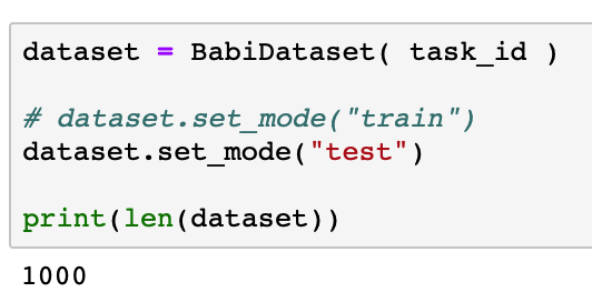
3、编写几行代码,探索一下在这个数据集中一个Task中训练集有多少条,测试集有多少条(提示是下面一个cell的代码)
dataset = BabiDataset( task_id )

# dataset.set_mode("train")
dataset.set_mode("test")

print(len(dataset))
1000
9000 observations in training set.
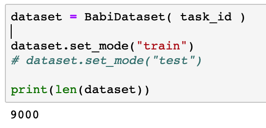
1000 observations in test set.
4、根据注释提示,将input module中的bi-directional GRU改成普通的GRU,重新运行网络。
Three adaptations:
InputModule.gru = nn.GRU(hidden_size, hidden_size, bidirectional=True, batch_first=True)$\to$InputModule.gru = nn.GRU(hidden_size, hidden_size, bidirectional=False, batch_first=True).h0 = Variable(torch.zeros(1, batch_num, self.hidden_size).cuda())$\to$h0 = Variable(torch.zeros(1, batch_num, self.hidden_size).cuda()).- Comment
facts = facts[:, :, :self.hidden_size] + facts[:, :, self.hidden_size:].
The neural network is recompile as above.
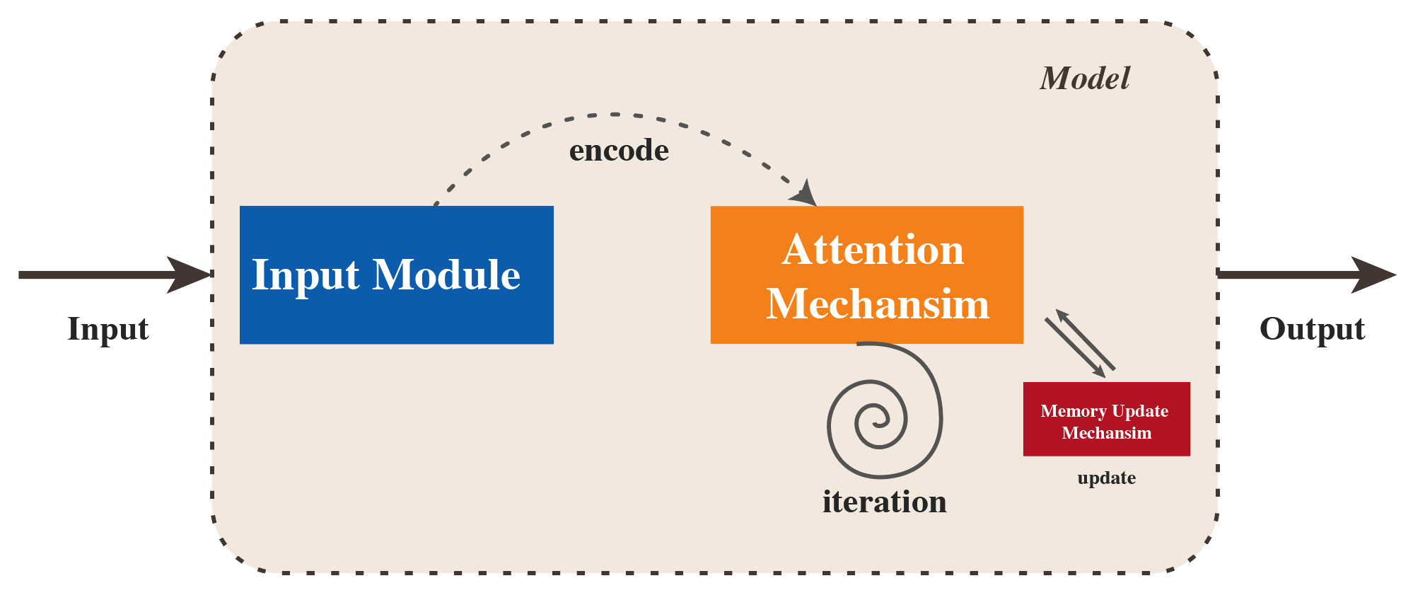
5、根据代码和理解,用自己的语言简要描述Episodic Memory所进行的操作。
Pisodic Memory is composed of Internal Memory, Memory Update Mechansim and Attention Mechansim. Information encoded by Input Module is input into the Attention Mechanism to search for related information for several iterations, during which the Memory Update Mechanism updates memory and finally outputs the answer. The flow chart of this model is shown as follows: